HoloViz Python dashboards for ocean data from diving, autonomous floats

Emilio Mayorga
Senior Oceanographer
Applied Physics Laboratory
University of Washington, Seattle
emiliomayorga@gmail.com


CUGOS Monthly Meeting, 2025-04-16

My excuse for talking about ...

  • A specific type of data I'm working with.
  • The (Python) tools I'm using to pre-process data and for ...
  • Developing custom data exploration web applications (dashboards).

Hopefully just enough details to whet your appetite!

Specifically

  • Depth-profiling (diving) floats, and their data
  • The HoloViz ecosystem of interrelated Python packages for interactive data visualization and web app development
  • Two* specific examples (two projects) with dashboards for such data

* Maybe 3 ...

Depth-profiling (diving) floats

  • Largely passive, not self-propelled
  • Buoyancy is controlled by changing its density via a bladder that's contracted (lower volume -> higher density -> sinking) or expanded (ascending)
  • At the surface, transmits data and receives instructions via satellite
  • Latitude and longitude positions (from GPS) available only when float surfaces
  • May be "nudged" towards a target path by adjusting 2 parameters at each "dive": what depth to "park" at, and for how long

Argo floats & Argo network

Most widespread type and use are the "Argo" floats that are part of the global Argo network (https://argo.ucsd.edu). They feature a standard set of sensors, follow a fixed descending-and-ascending behavior, and feed into a common data system. Data are openly available

Argo global deployments status

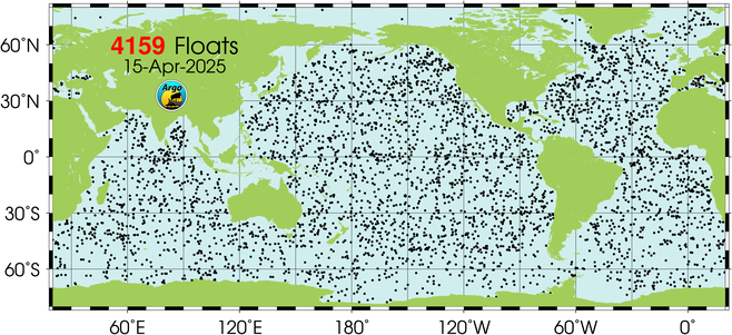
These projects are not feeding data to Argo, yet.

Depth-profiling floats

Profiling floats, profile navigation behavior

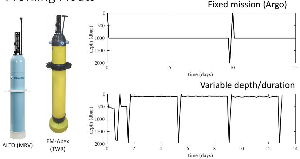
1 dbar (decibar, pressure) is approx. 1 meter. EM-APEX floats also measure current velocity.

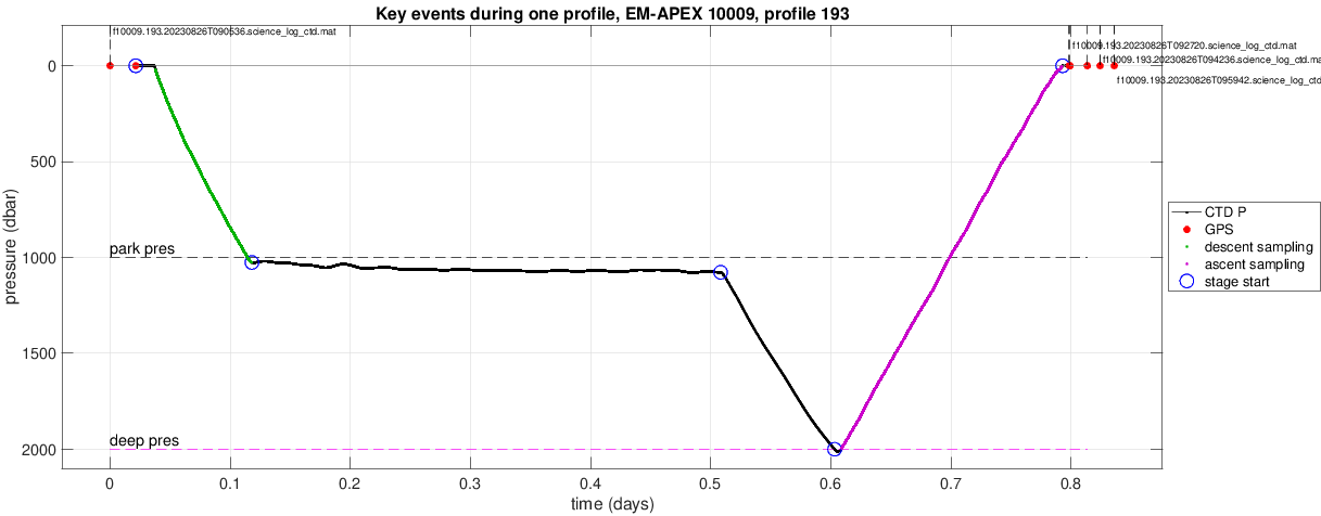
Components of a dive

Components and events from a float dive

Two projects: SQUID and ALFAC

  • SQUID: Sampling QUantitative Internal-wave Distributions
  • ALFAC: Array of Lagrangian Floats for Areal Coverage

Will try to share the code for both apps on GitHub in the future. But it'll take some work
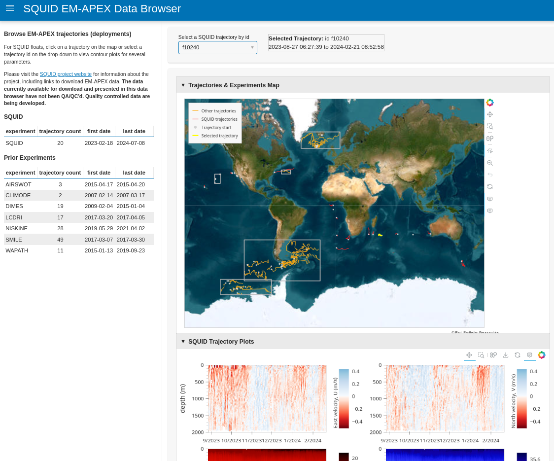
Projects: SQUID

  • https://www.apl.uw.edu/project/project.php?id=squid. Led by James Girton, APL
  • Its goal is "to improve the broad-scale characterization of internal wave climates through global deployments of autonomous profiling floats measuring shear, strain, and turbulent mixing". And to develop data standards and mechanisms to make data from EM-APEX floats more widely accessible and shareable.
  • Deployments around the world
  • HoloViz/Panel app: https://squid-test1.azurewebsites.net
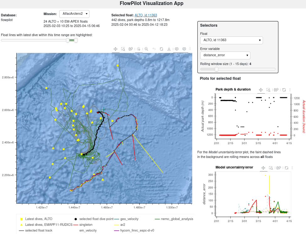
Projects: ALFAC

  • No public website. Led by Zoltan Szuts, APL
  • Developing a "shoreside autonomy software, 'FlowPilot', that selects dive parameters (park depth & duration) to align with ocean currents favorable to the chosen sampling mission. FlowPilot uses in-situ float data and external data sources to predict float drift paths using multiple prediction methods, evaluates the prediction uncertainties, and makes a recommendation for the next dive in real-time."
  • Deployment of clusters of floats within specific areas, for experiments. So far, in the Western Pacific and Gulf Stream.
  • HoloViz/Panel app is for internal use only at this time

HoloViz ecosystem of packages, https://holoviz.org

HoloViz packages

  • "a set of open-source Python packages to streamline the entire process of working with small and large datasets [for visualization and exploration] in a web browser"
  • Run from scripts/modules or Jupyter notebook
  • Support different plotting backends (matplotlib, plotly, etc), but bokeh is more "native"
  • Apps usually require server deployment and Python environment, but light-weight apps may be client-side
  • Great set of working tutorials and examples, for individual packages and integrated scenarios. https://holoviz.org/tutorial/
  • I will focus on: Panel, HoloViews, GeoViews, hvPlot, param

Explore HoloViews, GeoViews and hvPlot

With a built-in Panel app (hvplot.explorer) on the side

In [1]:
from pathlib import Path
import geopandas as gpd
import pandas as pd
import hvplot.pandas # noqa
import warnings
warnings.simplefilter("ignore", category=UserWarning)

data_dpth = Path("./data")
In [2]:
trajectories_gdf = gpd.read_parquet(data_dpth / "gps_deployments_lines_allexperiments.geoparquet")

trajectories_start_gdf = trajectories_gdf.set_geometry('point_start_geom').drop(columns='geometry')

# Default GeoDataFrame plotting with matplotlib: trajectories_start_gdf.plot()
trajectories_start_gdf.hvplot()
Out[2]:
In [3]:
# Customize a bit
trajectories_start_gdf.hvplot(
    geo=True,
    by='experiment', 
    hover_cols=['deployment', 'datetime_min'], 
    tiles='EsriNatGeo',
    tools=['undo', 'hover'],
)
Out[3]:
In [4]:
# Out-of-the-box hvplot explorer
pd.DataFrame(trajectories_start_gdf).hvplot.explorer()
Out[4]:
In [5]:
# Fall back to Geo/HoloViews. See "overlay" (*) and "layout" (+) operators
import geoviews as gv, holoviews as hv
hv.extension('bokeh')

basemaptiles = gv.tile_sources.EsriOceanBase
trajectories_start = gv.Points(trajectories_start_gdf)

trajectories_start + trajectories_gdf.hvplot(geo=True)
# Now fancier, with tiles and holoviews "options"
# ( (basemaptiles * trajectories_start.opts(tools=['hover'])).opts(xlabel='lat', ylabel='lon', title="with holoviews")
#   + trajectories_gdf.hvplot(geo=True, tiles='OSM', title='with hvplot')
# )
No description has been provided for this image No description has been provided for this image
Out[5]:
In [6]:
import hvplot.xarray
import xarray as xr

xr_ds = xr.tutorial.open_dataset('air_temperature').load()
xr_ds

# -- Alternatively, can play with this Zarr dataset accessed from the cloud
# From https://pangeo-forge.org/dashboard/feedstock/78
# zarr_store = 'https://ncsa.osn.xsede.org/Pangeo/pangeo-forge/pangeo-forge/AGDC-feedstock/AGCD.zarr'
# xr_ds = xr.open_dataset(zarr_store, engine='zarr', chunks={})
# Lazy loading (metadata and coordinate values only)
# Data variables loaded as lazy, chunked "Dask" arrays
# print(f"Total size (not downloaded size!): {xr_ds.nbytes/1e9:.1f} GB")
# xr_ds
Out[6]:
<xarray.Dataset> Size: 31MB
Dimensions:  (lat: 25, time: 2920, lon: 53)
Coordinates:
  * lat      (lat) float32 100B 75.0 72.5 70.0 67.5 65.0 ... 22.5 20.0 17.5 15.0
  * lon      (lon) float32 212B 200.0 202.5 205.0 207.5 ... 325.0 327.5 330.0
  * time     (time) datetime64[ns] 23kB 2013-01-01 ... 2014-12-31T18:00:00
Data variables:
    air      (time, lat, lon) float64 31MB 241.2 242.5 243.5 ... 296.2 295.7
Attributes:
    Conventions:  COARDS
    title:        4x daily NMC reanalysis (1948)
    description:  Data is from NMC initialized reanalysis\n(4x/day).  These a...
    platform:     Model
    references:   http://www.esrl.noaa.gov/psd/data/gridded/data.ncep.reanaly...
xarray.Dataset
    • lat: 25
    • time: 2920
    • lon: 53
    • lat
      (lat)
      float32
      75.0 72.5 70.0 ... 20.0 17.5 15.0
      standard_name :
      latitude
      long_name :
      Latitude
      units :
      degrees_north
      axis :
      Y
      array([75. , 72.5, 70. , 67.5, 65. , 62.5, 60. , 57.5, 55. , 52.5, 50. , 47.5,
             45. , 42.5, 40. , 37.5, 35. , 32.5, 30. , 27.5, 25. , 22.5, 20. , 17.5,
             15. ], dtype=float32)
    • lon
      (lon)
      float32
      200.0 202.5 205.0 ... 327.5 330.0
      standard_name :
      longitude
      long_name :
      Longitude
      units :
      degrees_east
      axis :
      X
      array([200. , 202.5, 205. , 207.5, 210. , 212.5, 215. , 217.5, 220. , 222.5,
             225. , 227.5, 230. , 232.5, 235. , 237.5, 240. , 242.5, 245. , 247.5,
             250. , 252.5, 255. , 257.5, 260. , 262.5, 265. , 267.5, 270. , 272.5,
             275. , 277.5, 280. , 282.5, 285. , 287.5, 290. , 292.5, 295. , 297.5,
             300. , 302.5, 305. , 307.5, 310. , 312.5, 315. , 317.5, 320. , 322.5,
             325. , 327.5, 330. ], dtype=float32)
    • time
      (time)
      datetime64[ns]
      2013-01-01 ... 2014-12-31T18:00:00
      standard_name :
      time
      long_name :
      Time
      array(['2013-01-01T00:00:00.000000000', '2013-01-01T06:00:00.000000000',
             '2013-01-01T12:00:00.000000000', ..., '2014-12-31T06:00:00.000000000',
             '2014-12-31T12:00:00.000000000', '2014-12-31T18:00:00.000000000'],
            shape=(2920,), dtype='datetime64[ns]')
    • air
      (time, lat, lon)
      float64
      241.2 242.5 243.5 ... 296.2 295.7
      long_name :
      4xDaily Air temperature at sigma level 995
      units :
      degK
      precision :
      2
      GRIB_id :
      11
      GRIB_name :
      TMP
      var_desc :
      Air temperature
      dataset :
      NMC Reanalysis
      level_desc :
      Surface
      statistic :
      Individual Obs
      parent_stat :
      Other
      actual_range :
      [185.16 322.1 ]
      array([[[241.2 , 242.5 , 243.5 , ..., 232.8 , 235.5 , 238.6 ],
              [243.8 , 244.5 , 244.7 , ..., 232.8 , 235.3 , 239.3 ],
              [250.  , 249.8 , 248.89, ..., 233.2 , 236.39, 241.7 ],
              ...,
              [296.6 , 296.2 , 296.4 , ..., 295.4 , 295.1 , 294.7 ],
              [295.9 , 296.2 , 296.79, ..., 295.9 , 295.9 , 295.2 ],
              [296.29, 296.79, 297.1 , ..., 296.9 , 296.79, 296.6 ]],
      
             [[242.1 , 242.7 , 243.1 , ..., 232.  , 233.6 , 235.8 ],
              [243.6 , 244.1 , 244.2 , ..., 231.  , 232.5 , 235.7 ],
              [253.2 , 252.89, 252.1 , ..., 230.8 , 233.39, 238.5 ],
              ...,
              [296.4 , 295.9 , 296.2 , ..., 295.4 , 295.1 , 294.79],
              [296.2 , 296.7 , 296.79, ..., 295.6 , 295.5 , 295.1 ],
              [296.29, 297.2 , 297.4 , ..., 296.4 , 296.4 , 296.6 ]],
      
             [[242.3 , 242.2 , 242.3 , ..., 234.3 , 236.1 , 238.7 ],
              [244.6 , 244.39, 244.  , ..., 230.3 , 232.  , 235.7 ],
              [256.2 , 255.5 , 254.2 , ..., 231.2 , 233.2 , 238.2 ],
              ...,
      ...
              [294.79, 295.29, 297.49, ..., 295.49, 295.39, 294.69],
              [296.79, 297.89, 298.29, ..., 295.49, 295.49, 294.79],
              [298.19, 299.19, 298.79, ..., 296.09, 295.79, 295.79]],
      
             [[245.79, 244.79, 243.49, ..., 243.29, 243.99, 244.79],
              [249.89, 249.29, 248.49, ..., 241.29, 242.49, 244.29],
              [262.39, 261.79, 261.29, ..., 240.49, 243.09, 246.89],
              ...,
              [293.69, 293.89, 295.39, ..., 295.09, 294.69, 294.29],
              [296.29, 297.19, 297.59, ..., 295.29, 295.09, 294.39],
              [297.79, 298.39, 298.49, ..., 295.69, 295.49, 295.19]],
      
             [[245.09, 244.29, 243.29, ..., 241.69, 241.49, 241.79],
              [249.89, 249.29, 248.39, ..., 239.59, 240.29, 241.69],
              [262.99, 262.19, 261.39, ..., 239.89, 242.59, 246.29],
              ...,
              [293.79, 293.69, 295.09, ..., 295.29, 295.09, 294.69],
              [296.09, 296.89, 297.19, ..., 295.69, 295.69, 295.19],
              [297.69, 298.09, 298.09, ..., 296.49, 296.19, 295.69]]],
            shape=(2920, 25, 53))
    • lat
      PandasIndex
      PandasIndex(Index([75.0, 72.5, 70.0, 67.5, 65.0, 62.5, 60.0, 57.5, 55.0, 52.5, 50.0, 47.5,
             45.0, 42.5, 40.0, 37.5, 35.0, 32.5, 30.0, 27.5, 25.0, 22.5, 20.0, 17.5,
             15.0],
            dtype='float32', name='lat'))
    • lon
      PandasIndex
      PandasIndex(Index([200.0, 202.5, 205.0, 207.5, 210.0, 212.5, 215.0, 217.5, 220.0, 222.5,
             225.0, 227.5, 230.0, 232.5, 235.0, 237.5, 240.0, 242.5, 245.0, 247.5,
             250.0, 252.5, 255.0, 257.5, 260.0, 262.5, 265.0, 267.5, 270.0, 272.5,
             275.0, 277.5, 280.0, 282.5, 285.0, 287.5, 290.0, 292.5, 295.0, 297.5,
             300.0, 302.5, 305.0, 307.5, 310.0, 312.5, 315.0, 317.5, 320.0, 322.5,
             325.0, 327.5, 330.0],
            dtype='float32', name='lon'))
    • time
      PandasIndex
      PandasIndex(DatetimeIndex(['2013-01-01 00:00:00', '2013-01-01 06:00:00',
                     '2013-01-01 12:00:00', '2013-01-01 18:00:00',
                     '2013-01-02 00:00:00', '2013-01-02 06:00:00',
                     '2013-01-02 12:00:00', '2013-01-02 18:00:00',
                     '2013-01-03 00:00:00', '2013-01-03 06:00:00',
                     ...
                     '2014-12-29 12:00:00', '2014-12-29 18:00:00',
                     '2014-12-30 00:00:00', '2014-12-30 06:00:00',
                     '2014-12-30 12:00:00', '2014-12-30 18:00:00',
                     '2014-12-31 00:00:00', '2014-12-31 06:00:00',
                     '2014-12-31 12:00:00', '2014-12-31 18:00:00'],
                    dtype='datetime64[ns]', name='time', length=2920, freq=None))
  • Conventions :
    COARDS
    title :
    4x daily NMC reanalysis (1948)
    description :
    Data is from NMC initialized reanalysis (4x/day). These are the 0.9950 sigma level values.
    platform :
    Model
    references :
    http://www.esrl.noaa.gov/psd/data/gridded/data.ncep.reanalysis.html
In [7]:
xr_ds['air'].sel(time='2013-06-01 12:00').hvplot()
Out[7]:
In [8]:
# Let hvplot create a slider widget to interactively flip through time
xr_ds['air'].hvplot(groupby='time')
Out[8]:

Quick Panel demo

Define a couple of Panel widgets and link them to a dataset via .interactive() method

Demo taken from https://hvplot.holoviz.org

In [9]:
import panel as pn

w_quantile = pn.widgets.FloatSlider(name='quantile', start=0, end=1)
w_time = pn.widgets.IntSlider(name='time', start=0, end=10)

(  xr_ds['air'].interactive(loc='left')
   .isel(time=w_time)
   .quantile(q=w_quantile, dim='lon')
   .hvplot(ylabel='Air Temperature [K]', width=500) )
Out[9]:

Source data structure and formats

SQUID: source netCDF file and pre-processed GeoParquet files

  • (Geo)Parquet: open "columnar" data store with chunking and compression, plays well in cloud object storage
  • Pre-processing done with xarray, GeoPandas.
  • GeoParquet file generated from source netCDF file, to extract point and lat-lon line geometries and aggregated attributes, for quick & convenient access in the SQUID App.
  • That's the gps_deployments_lines_allexperiments.geoparquet file used earlier in the hvPlot demo. Includes both line and point geometry columns.

SQUID: binned netCDF file, with several float "trajectories"

  • A data product heavily post-processed through scripts that could be fully automated.
  • Not a regular grid structure; a "discrete sampling geometries" feature type, per netCDF data model.
  • Open the netCDF file with xarray, examine its structure.
In [11]:
zgrid_ds = xr.open_dataset(data_dpth / "SQUID_NCEI.nc", decode_times=False)
zgrid_ds
Out[11]:
<xarray.Dataset> Size: 600MB
Dimensions:     (trajectory: 20, obs: 234, z: 2001, trid_len: 6)
Coordinates:
  * trajectory  (trajectory) int32 80B 1 2 3 4 5 6 7 8 ... 14 15 16 17 18 19 20
    time        (obs, trajectory) float64 37kB ...
    lat         (obs, trajectory) float64 37kB ...
    lon         (obs, trajectory) float64 37kB ...
Dimensions without coordinates: obs, z, trid_len
Data variables: (12/17)
    depth       (z) float64 16kB ...
    T           (z, obs, trajectory) float64 75MB ...
    S           (z, obs, trajectory) float64 75MB ...
    P           (z, obs, trajectory) float64 75MB ...
    U           (z, obs, trajectory) float64 75MB ...
    V           (z, obs, trajectory) float64 75MB ...
    ...          ...
    flid        (trajectory) int32 80B ...
    trid        (trid_len, trajectory) |S1 120B ...
    pid         (obs, trajectory) float64 37kB ...
    hpid        (obs, trajectory) float64 37kB ...
    depl        (trajectory) int32 80B ...
    EM-APEX     float64 8B ...
Attributes: (12/26)
    ncei_template_version:      NCEI_NetCDF_TrajectoryProfile_Incomplete_Temp...
    featureType:                trajectoryProfile
    title:                      T, S, U, V and derived quantities measured by...
    summary:                    T, S, potential density, N^2, U, V, u_z, and ...
    Conventions:                CF-1.6, ACDD-1.3
    acknowledgments:            NOPP Global Internal Wave Project. Funding fr...
    ...                         ...
    geospatial_lat_units:       degree_north
    geospatial_lon_units:       degree_east
    geospatial_vertical_units:  meters
    platform:                   EM-APEX
    references:                 
    comment:                    Deployed from multiple cruises of opportunity...
xarray.Dataset
    • trajectory: 20
    • obs: 234
    • z: 2001
    • trid_len: 6
    • trajectory
      (trajectory)
      int32
      1 2 3 4 5 6 7 ... 15 16 17 18 19 20
      long_name :
      Unique identifier for each feature instance
      cf_role :
      trajectory_id
      comment :
      ID number of Float-Deployment pair
      array([ 1,  2,  3,  4,  5,  6,  7,  8,  9, 10, 11, 12, 13, 14, 15, 16, 17, 18,
             19, 20], dtype=int32)
    • time
      (obs, trajectory)
      float64
      ...
      long_name :
      Time, UTC
      standard_name :
      time
      units :
      seconds since 1970-01-01 00:00:00 0:00
      calendar :
      Julian
      axis :
      T
      [4680 values with dtype=float64]
    • lat
      (obs, trajectory)
      float64
      ...
      long_name :
      mean latitude of EM-APEX profiles
      standard_name :
      latitude
      units :
      degree_north
      axis :
      Y
      valid_min :
      -45.5395
      valid_max :
      37.1694
      comment :
      Mean latitude during each float dive
      Coordinates :
      time lat lon
      [4680 values with dtype=float64]
    • lon
      (obs, trajectory)
      float64
      ...
      long_name :
      mean longitude of EM-APEX profiles
      standard_name :
      longitude
      units :
      degree_east
      axis :
      X
      valid_min :
      -125.105
      valid_max :
      93.4306
      comment :
      Mean longitude during each float dive
      Coordinates :
      time lat lon
      [4680 values with dtype=float64]
    • depth
      (z)
      float64
      ...
      long_name :
      depths of gridded EM-APEX profiles
      standard_name :
      depth
      units :
      meters [m]
      axis :
      Z
      positive :
      down
      valid_min :
      0
      valid_max :
      2000
      comment :
      Profile depths interpolated to common grid
      [2001 values with dtype=float64]
    • T
      (z, obs, trajectory)
      float64
      ...
      long_name :
      gridded EM-APEX temperature
      standard_name :
      sea_water_temperature
      units :
      Kelvin
      platform_variable :
      EM_APEX
      instrument :
      thermistor
      [9364680 values with dtype=float64]
    • S
      (z, obs, trajectory)
      float64
      ...
      long_name :
      gridded EM-APEX salinity
      standard_name :
      sea_water_salinity
      units :
      1e-3
      platform_variable :
      EM_APEX
      comment :
      Units are standard psu. The units refered to in Units attribute refer to the CF Convention for standard name and units.
      [9364680 values with dtype=float64]
    • P
      (z, obs, trajectory)
      float64
      ...
      long_name :
      gridded EM-APEX pressure derived from depth and latitude
      standard_name :
      sea_water_pressure
      units :
      decibar
      platform_variable :
      EM_APEX
      [9364680 values with dtype=float64]
    • U
      (z, obs, trajectory)
      float64
      ...
      long_name :
      gridded EM-APEX east velocity component
      standard_name :
      eastward_sea_water_velocity
      units :
      meter per second
      platform_variable :
      EM_APEX
      instrument :
      EM-APEX
      [9364680 values with dtype=float64]
    • V
      (z, obs, trajectory)
      float64
      ...
      long_name :
      gridded EM-APEX north velocity component
      standard_name :
      northward_sea_water_velocity
      units :
      meter per second
      platform_variable :
      EM_APEX
      instrument :
      EM-APEX
      [9364680 values with dtype=float64]
    • chi1
      (z, obs, trajectory)
      float64
      ...
      long_name :
      temperature_variance_dissipation
      units :
      degree Celsius square per second
      platform_variable :
      EM_APEX
      comment :
      Rate of dissipation of temperature variance measured by Probe 1
      [9364680 values with dtype=float64]
    • chi2
      (z, obs, trajectory)
      float64
      ...
      long_name :
      temperature_variance_dissipation
      units :
      degree Celsius square per second
      platform_variable :
      EM_APEX
      comment :
      Rate of dissipation of temperature variance measured by Probe 2
      [9364680 values with dtype=float64]
    • ptime
      (z, obs, trajectory)
      float64
      ...
      long_name :
      time_along_profile
      units :
      seconds since 1970-01-01 00:00:00 0:00
      calendar :
      Julian
      platform_variable :
      EM_APEX
      [9364680 values with dtype=float64]
    • U0
      (obs, trajectory)
      float64
      ...
      long_name :
      Drift eastward velocity of a float while at surface
      standard_name :
      surface eastward velocity
      units :
      meter per second
      Coordinates :
      time lat lon
      [4680 values with dtype=float64]
    • V0
      (obs, trajectory)
      float64
      ...
      long_name :
      Drift northward velocity of a float while at surface
      standard_name :
      surface northward velocity
      units :
      meter per second
      Coordinates :
      time lat lon
      [4680 values with dtype=float64]
    • flid
      (trajectory)
      int32
      ...
      long_name :
      EM-APEX float id number
      standard_name :
      Float id number
      [20 values with dtype=int32]
    • trid
      (trid_len, trajectory)
      |S1
      ...
      long_name :
      Trajectory id
      comment :
      A 2-dimensional character array representing a unique trajectory id string per float deployment. The rendering of this trajectory id is dependent on the software used to read the netcdfs. If the trajectory id does not look like a composition of a float number and characters (e.g. 'f9436', '7805s2'), try to compose the trajectory id string by concatenating the characters over the trid_len dimension
      [120 values with dtype=|S1]
    • pid
      (obs, trajectory)
      float64
      ...
      long_name :
      Profile id number
      comment :
      Profile number, where a profile consist of a full down + up cycle
      [4680 values with dtype=float64]
    • hpid
      (obs, trajectory)
      float64
      ...
      long_name :
      Half-profile id number
      comment :
      A Half profile consist of either a down or up profile. Odd number are down-profiles, even numbers are up-profiles
      [4680 values with dtype=float64]
    • depl
      (trajectory)
      int32
      ...
      long_name :
      Deployment number of a float
      standard_name :
      deployment
      comment :
      Deployment number within an experiment. An experiment can have a single deployment or multiple deployments where all or part of the float array are deployed.
      [20 values with dtype=int32]
    • EM-APEX
      ()
      float64
      ...
      long_name :
      EM-APEX
      wmo_code :
      [1 values with dtype=float64]
    • trajectory
      PandasIndex
      PandasIndex(Index([1, 2, 3, 4, 5, 6, 7, 8, 9, 10, 11, 12, 13, 14, 15, 16, 17, 18, 19, 20], dtype='int32', name='trajectory'))
  • ncei_template_version :
    NCEI_NetCDF_TrajectoryProfile_Incomplete_Template_v2.0
    featureType :
    trajectoryProfile
    title :
    T, S, U, V and derived quantities measured by EM-APEX during SQUIDexperiment
    summary :
    T, S, potential density, N^2, U, V, u_z, and v_z measured by EM-APEX float and interpolated onto a common depth grid
    Conventions :
    CF-1.6, ACDD-1.3
    acknowledgments :
    NOPP Global Internal Wave Project. Funding from the National Science Foundation (OCE-2232796)
    date_created :
    23-Jul-2024 09:14:39
    creator_name :
    James Girton, Aurelie Moulin
    creator_email :
    girton@uw.edu, amoulin@uw.edu
    Institution :
    Applied Physics Laboratory - University of Washington
    geospatial_lat_min :
    -59.1682 (>0, N; <0, S)
    geospatial_lat_max :
    40.8682 (>0, N; <0, S)
    geospatial_lon_min :
    -159.1725 (>0, E; <0, W)
    geospatial_lon_max :
    155.869 (>0, E; <0, W)
    vertical_min :
    0.0
    vertical_max :
    2000.0
    vertical_positive :
    up
    time_coverage_start :
    18-Feb-2023 21:11:05
    time_coverage_end :
    09-Jul-2024 00:16:00
    sea_name :
    Multiple
    geospatial_lat_units :
    degree_north
    geospatial_lon_units :
    degree_east
    geospatial_vertical_units :
    meters
    platform :
    EM-APEX
    references :
    comment :
    Deployed from multiple cruises of opportunity worlwide for the Sampling Quantitative Internal Waves Dissipation project (SQUID)starting in Feb 2023. PI: James Girton (girton@uw.edu)

ALFAC: FlowPilot Database (PostgreSQL)

Complete ERD; tables used by FP Viz app are in green

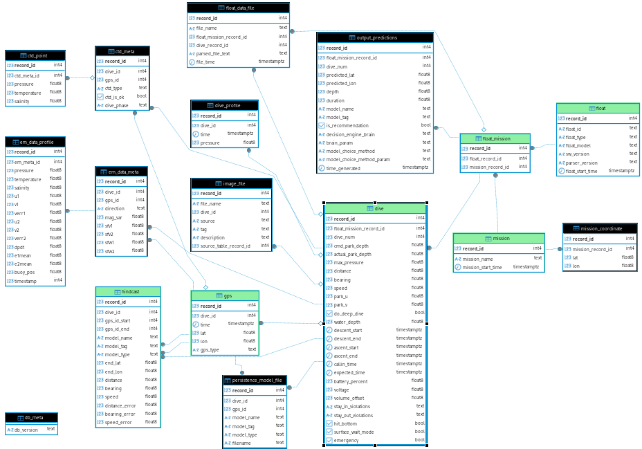
Tables used by the FlowPilot Visualization App

ERD, tables used by FP Viz app

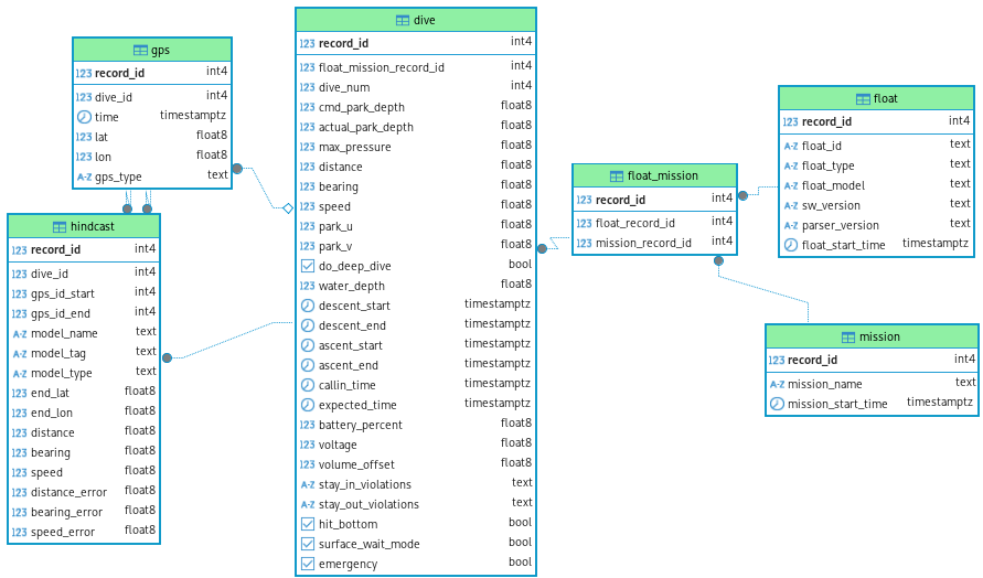
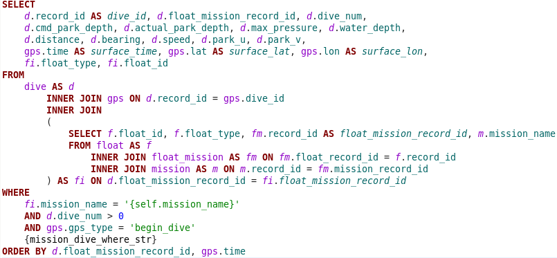
Sample SQL for pre-processing, for viz app

For dive data. SQL code trimmed a bit. Pulled in from DB via pandas.read_sql_query(). This is followed by a lot of additional processing: further data cleaning, timestamp formatting, creating point and line GeoDataFrames, creating dynamic HoloViews elements, etc.

SQL code for querying dives

The apps

Or at least screenshots

SQUID

SQUID App screenshot

ALFAC / FlowPilot

ALFAC FlowPilot Visualization App screenshot

HoloViz code snippets from my apps

Select a "trajectory" based on change to a text widget, trajectory_sel_text. The .apply() method in action, passing a param object.

def select_by_trid(hvds, trajectory_id):    
    return hvds.select(trajectory_id=trajectory_id)

selected_trajectory_layer = (
    gps_deployments_hvPath.relabel("Selected trajectory").apply(
        select_by_trid, 
        trajectory_id=trajectory_sel_text.param.value,
    ).opts(color='yellow', line_width=3)
)

Update the trajectory_sel_text Panel text widget based on a selection ("tap") action on gps_deployments_hvPath line element.

traj_stream = Selection1D(source=gps_deployments_hvPath, index=[0])

@pn.depends(s=traj_stream.param.index, watch=True)
def _update_traj_select(s):
    select_index = s[0] if s else 0
    trajectory_sel_text.value = traj_lines_trajid_vs_idx[select_index]

Use CSS and styling properties to heavily customiz appearance and rendering of a Panel element.

MARKDOWN_CSS = """
p {  margin: 1px; padding-top: 0px; padding-bottom: 0px;
     border: 0.5px solid #cccccc; font-size: 11pt;  }
"""
sel_trajectory_pn_md = pn.pane.Markdown(
    sel_traj_display_str(trajectory_id_initial),
    styles={'padding-top': '0px', 'padding-bottom': '0px'},
    stylesheets=[MARKDOWN_CSS]
)

Arrange app elements using Panel Row and Col elements

header_bar_mission_col = pn.Column(
    pn.Row(
        fpv_md.header_bar_mission,
        fpv_widgets.mission_select),
    pn.Row(
        fpv_md.header_bar_mission_info,
        margin=0),
    margin=0, width=260,
)

Use a Panel web framework template.

app_template = pn.template.FastListTemplate(
    title=title_str, sidebar_width=400,
    sidebar=[pn.pane.Markdown(description_md), pn.pane.Markdown("### SQUID")],
    main=[pn.Row(traj_sel_text, sel_traj_pn_md,
           align='center', margin=0, styles={'padding-top': '0px'}),
          plots_accordion],
    theme_toggle=False, background='lightgray'
)

Running the app

  • Within the app code, use my_panel_app_object.servable() (or my_panel_app_object.servable().show() for testing).
  • From command line: panel serve --autoreload --global-loading-spinner --port 5100 --allow-websocket-origin='*' --log-file mylogfile.log basepath/myappnotebook.ipynb
    • Bare bones: panel serve basepath/myappnotebook.ipynb

App deployment

  • SQUID
    • MS Azure (using Ubuntu Linux). https://squid-test1.azurewebsites.net
    • Maintained and developed in a local git clone
    • Updates deployed via Azure Git push. Python environment maitained via pip (or Docker container, but I wanted to keep things simple)
    • Project page https://www.apl.uw.edu/project/project.php?id=squid
  • ALFAC
    • Everything is in APL network only, behind VPN
    • Deployment to an Ubuntu server, with Apache
    • Maintained and developed via project GitLab.
    • Updates deployed via Git pull from GitLab repo
  • TROCAS
    • CO2 at the mouth of the Amazon River, sampled continuously by boat
    • On GitHub, https://github.com/amazon-riverbgc/trocas-herokuapp1. But the code is getting long in the tooth!
    • Deployment to Heroku via Heroku CLI, as Docker container
    • See https://amazon-riverbgc.github.io/TROCAS/docs/databrowser.html

Strengths and especially annoyances

For a later time .... Sigh

Ask me today or ping me any time.

In [ ]: