Niveles de agua del Lago Cocibolca basado en altimetria satelital
VER LA VERSION DE DESARROLLO PARA APUNTES Y PARTES EXPERIMENTALES
Actualizacion: 4/25
TAREAS:
Para esta version final nada mas. Para otras tareas, ver la version de desarrollo.
Remover partes mas exploratorias
Definir y utilizar una cabecera (header) estandard, en una celda, con mi nombre, enlace (a github?), fecha, enlace al sitio Jupyter Book, etc.
Tambien un footnote con versiones de los paquetes y enlaces al archivo yaml de conda env?
HECHO. Orden a seguir:
Leer el paso satelital y visualizar en un mapa
Acceder e ingerir los datos de niveles de agua
Pre-procesar y suplementar los datos ingeridos
Explorar patrones temporales
Explorar lakepy (incluyendo el Xolotlan)
Introduccion
Metas de este cuaderno
Un poco sobre datos altimetricos y G-REALM
Importar paquetes
Los que se usan mas ampliamente, aqui. Los mas especificos, en sus secciones correspondientes
import warnings

import numpy as np
import pandas as pd
import matplotlib
import matplotlib.pyplot as plt
import seaborn as sns
warnings.simplefilter('ignore')
matplotlib.style.use('ggplot')
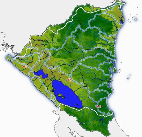
Leer el paso satelital y visualizar en un mapa
An-adir un enlace a mi tutorial sobre vectores en GHW19?
import geopandas as gpd
import folium
kmlurl = "https://ipad.fas.usda.gov/rssiws/ggeoxml/351_Nicaragua.kml"
gpd.io.file.fiona.drvsupport.supported_drivers['KML'] = 'rw'
See this good reference for reading KMLs and their complexities: https://gis.stackexchange.com/questions/328525/geopandas-read-file-only-reading-first-part-of-kml
gdf = gpd.read_file(kmlurl, driver='KML')
len(gdf)
190
gdf.tail()
| Name | Description | geometry | |
|---|---|---|---|
| 185 | POINT (-85.63035 0.00000) | ||
| 186 | POINT (-85.62943 0.00000) | ||
| 187 | POINT (-85.62851 0.00000) | ||
| 188 | POINT (-85.62759 0.00000) | ||
| 189 | Topex/Jason Pass | LINESTRING (-85.80074 11.56268, -85.79982 11.5... |
gdf.geometry.type.value_counts()
Point         189
LineString      1
dtype: int64
# usando folium.Figure para controlar el taman-o sin introducir "padding"
fig = folium.Figure(width='60%')
mapa = folium.Map(tiles='StamenTerrain').add_to(fig)

folium.GeoJson(
    gdf[gdf.Name == 'Topex/Jason Pass'].geometry,
    tooltip="Paso satelital Topex/Jason"
).add_to(mapa)

# Set the map extent (bounds) to the extent of the bounding box
mapa.fit_bounds(mapa.get_bounds())
mapa
Acceder e ingerir los datos de niveles de agua
datos_tipo = '1'    # '1' o '2'
crudos_o_lisos = '' # '' o '.smooth'

lago_id = '0351'
fname = f"lake{lago_id}.10d.{datos_tipo}{crudos_o_lisos}.txt"
fname
'lake0351.10d.1.txt'
url = f"https://ipad.fas.usda.gov/lakes/images/{fname}"
Try using
infer_datetime_formatordate_parser
Para usar los datos «crudos»:
Column 1: Satellite mission name
Column 2: Satellite repeat cycle
Column 3: Calendar year/month/day of along track observations traversing target
Column 4: Hour of day at mid point of along track pass traversing target
Column 5: Minutes of hour at mid point of along track pass traversing target
Column 6: Target height variation with respect to Jason-2 reference pass mean level (meters, default=999.99)
Column 7: Estimated error of target height variation with respect to reference mean level (meters, default=99.999)
Column 8: Mean along track Ku-band backscatter coefficient (decibels, default=999.99)
Column 9: Wet tropospheric correction applied to range observation (TMR=T/P radiometer, JMR=Jason-1 radiometer,
    AMR=Jason-2 and Jason-3 radiometer, ERA=ECMWF ERA Interim Reanalysis model, ECM=ECMWF Operational model,
    MER=MERRA model, MIX=combination, U/A=unavailable, N/A=not applicable)
Column 10: Ionosphere correction applied to range observation (GIM=GPS model, NIC=NIC09 model, DOR=DORIS,
    IRI=IRI2007 model, BNT=Bent model, MIX=combination, U/A=unavailable, N/A=not applicable)
Column 11: Dry tropospheric correction applied to range observation (ERA=ECMWF ERA Interim Reanalysis model,
    ECM=ECMWF Operational model, U/A=unavailable, N/A=not applicable)
Column 12: Instrument operating mode 1 (default=9)
Column 13: Instrument operating mode 2 (default=9)
Column 14: Flag for potential frozen surface (ice-on=1, ice-off or unknown=0)
Column 15: Target height variation in EGM2008 datum (meters above mean sea level, default=9999.99)
Column 16: Flag for data source (GDR=0, IGDR=1)
Para usar los datos «lisos» (smooth):
Column 1: Calendar year/month/day
Column 2: Hour of day
Column 3: Minute of hour
Column 4: Smoothed target height variation with respect to Jason-2 reference pass level (meters, default=999.99)
Column 5: Smoothed target height variation in EGM2008 datum (meters above mean sea level, default=9999.99)
nombres_cols = {
    '': ['satmision', 'satrepetciclo',
         'fecha', 'hora', 'minuto', 'nivel',
         'est_error_nivel', 'kuband_scattcoef', 'wettropcorr', 'ionoscorr', 'drytropcorr',
         'instr_opmod1', 'instr_opmod2', 'superfcongelada_flag',
         'nivel_egm2008',
         'fuente_flag'],
    '.smooth': ['fecha', 'hora', 'minuto',
                'nivel',
                'nivel_egm2008']
}

skiprows = {
    '1': {'':27, '.smooth':12},
    '2': {'':33, '.smooth':12}
}
df0 = pd.read_csv(
    url, index_col=False, sep='\s+',
    names=nombres_cols[crudos_o_lisos],
    skiprows=skiprows[datos_tipo][crudos_o_lisos]
)
len(df0)
1116
df0.tail(10)
| satmision | satrepetciclo | fecha | hora | minuto | nivel | est_error_nivel | kuband_scattcoef | wettropcorr | ionoscorr | drytropcorr | instr_opmod1 | instr_opmod2 | superfcongelada_flag | nivel_egm2008 | fuente_flag | |
|---|---|---|---|---|---|---|---|---|---|---|---|---|---|---|---|---|
| 1106 | JASN3 | 181 | 20210115 | 17 | 19 | 0.57 | 0.042 | 13.60 | AMR | GIM | ECM | 2 | 2 | 0 | 32.67 | 1 |
| 1107 | JASN3 | 182 | 20210125 | 15 | 18 | 0.54 | 0.042 | 13.29 | AMR | GIM | ECM | 2 | 2 | 0 | 32.64 | 1 |
| 1108 | JASN3 | 183 | 20210204 | 13 | 16 | 0.50 | 0.042 | 12.85 | AMR | GIM | ECM | 2 | 2 | 0 | 32.60 | 1 |
| 1109 | JASN3 | 184 | 20210214 | 11 | 15 | 0.31 | 0.042 | 13.96 | AMR | GIM | ECM | 2 | 2 | 0 | 32.41 | 1 |
| 1110 | JASN3 | 185 | 20210224 | 9 | 13 | 0.28 | 0.042 | 13.06 | AMR | GIM | ECM | 2 | 2 | 0 | 32.38 | 1 |
| 1111 | JASN3 | 186 | 20210306 | 7 | 12 | 0.17 | 0.042 | 13.70 | AMR | GIM | ECM | 2 | 2 | 0 | 32.27 | 1 |
| 1112 | JASN3 | 187 | 20210316 | 5 | 10 | 0.12 | 0.042 | 13.18 | AMR | GIM | ECM | 2 | 2 | 0 | 32.22 | 1 |
| 1113 | JASN3 | 188 | 20210326 | 3 | 9 | 0.09 | 0.042 | 12.95 | AMR | GIM | ECM | 2 | 2 | 0 | 32.19 | 1 |
| 1114 | JASN3 | 189 | 20210405 | 1 | 7 | -0.02 | 0.042 | 12.88 | AMR | GIM | ECM | 2 | 2 | 0 | 32.08 | 1 |
| 1115 | JASN3 | 190 | 20210414 | 23 | 6 | -0.10 | 0.042 | 13.75 | AMR | GIM | ECM | 2 | 2 | 0 | 32.00 | 1 |
Pre-procesar y suplementar los datos ingeridos
df = df0[(df0['fecha'] != 99999999) & (df0['nivel'] < 999)].copy()
len(df)
1085
# Time *must* be zero-padded in conversion from integer to string
df.insert(1, 'FechaTiempo',
          pd.to_datetime(
              df['fecha'].map(str)
              + df['hora'].map(lambda nbr: "{0:02d}".format(nbr))
              + df['minuto'].map(lambda nbr: "{0:02d}".format(nbr)),
              format='%Y%m%d%H%M')
         )
df.drop(['fecha', 'hora', 'minuto'], axis=1, inplace=True)
df.FechaTiempo.min(), df.FechaTiempo.max()
(Timestamp('1992-10-02 14:54:00'), Timestamp('2021-04-14 23:06:00'))
df.tail(15)
| satmision | FechaTiempo | satrepetciclo | nivel | est_error_nivel | kuband_scattcoef | wettropcorr | ionoscorr | drytropcorr | instr_opmod1 | instr_opmod2 | superfcongelada_flag | nivel_egm2008 | fuente_flag | |
|---|---|---|---|---|---|---|---|---|---|---|---|---|---|---|
| 1101 | JASN3 | 2020-11-27 03:26:00 | 176 | 0.82 | 0.042 | 13.96 | AMR | GIM | ECM | 2 | 2 | 0 | 32.92 | 1 |
| 1102 | JASN3 | 2020-12-07 01:25:00 | 177 | 0.79 | 0.042 | 14.44 | AMR | GIM | ECM | 2 | 2 | 0 | 32.89 | 1 |
| 1103 | JASN3 | 2020-12-16 23:23:00 | 178 | 0.75 | 0.042 | 14.61 | AMR | GIM | ECM | 2 | 2 | 0 | 32.85 | 1 |
| 1104 | JASN3 | 2020-12-26 21:22:00 | 179 | 0.67 | 0.042 | 13.27 | AMR | GIM | ECM | 2 | 2 | 0 | 32.77 | 1 |
| 1105 | JASN3 | 2021-01-05 19:21:00 | 180 | 0.66 | 0.042 | 13.51 | AMR | GIM | ECM | 2 | 2 | 0 | 32.76 | 1 |
| 1106 | JASN3 | 2021-01-15 17:19:00 | 181 | 0.57 | 0.042 | 13.60 | AMR | GIM | ECM | 2 | 2 | 0 | 32.67 | 1 |
| 1107 | JASN3 | 2021-01-25 15:18:00 | 182 | 0.54 | 0.042 | 13.29 | AMR | GIM | ECM | 2 | 2 | 0 | 32.64 | 1 |
| 1108 | JASN3 | 2021-02-04 13:16:00 | 183 | 0.50 | 0.042 | 12.85 | AMR | GIM | ECM | 2 | 2 | 0 | 32.60 | 1 |
| 1109 | JASN3 | 2021-02-14 11:15:00 | 184 | 0.31 | 0.042 | 13.96 | AMR | GIM | ECM | 2 | 2 | 0 | 32.41 | 1 |
| 1110 | JASN3 | 2021-02-24 09:13:00 | 185 | 0.28 | 0.042 | 13.06 | AMR | GIM | ECM | 2 | 2 | 0 | 32.38 | 1 |
| 1111 | JASN3 | 2021-03-06 07:12:00 | 186 | 0.17 | 0.042 | 13.70 | AMR | GIM | ECM | 2 | 2 | 0 | 32.27 | 1 |
| 1112 | JASN3 | 2021-03-16 05:10:00 | 187 | 0.12 | 0.042 | 13.18 | AMR | GIM | ECM | 2 | 2 | 0 | 32.22 | 1 |
| 1113 | JASN3 | 2021-03-26 03:09:00 | 188 | 0.09 | 0.042 | 12.95 | AMR | GIM | ECM | 2 | 2 | 0 | 32.19 | 1 |
| 1114 | JASN3 | 2021-04-05 01:07:00 | 189 | -0.02 | 0.042 | 12.88 | AMR | GIM | ECM | 2 | 2 | 0 | 32.08 | 1 |
| 1115 | JASN3 | 2021-04-14 23:06:00 | 190 | -0.10 | 0.042 | 13.75 | AMR | GIM | ECM | 2 | 2 | 0 | 32.00 | 1 |
Hay que averiguar porque los datos terminan en Octubre.
df['año'] = df.FechaTiempo.dt.year
df['mes'] = df.FechaTiempo.dt.month
df['dia'] = df.FechaTiempo.dt.day
df['dda'] = df.FechaTiempo.dt.dayofyear
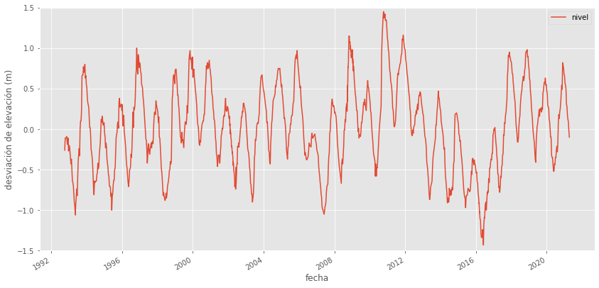
Explorar patrones temporales
df.plot(x='FechaTiempo', y='nivel', ylim=(-1.5, 1.5), figsize=(14, 7))
plt.ylabel('desviación de elevación (m)')
plt.xlabel('fecha');
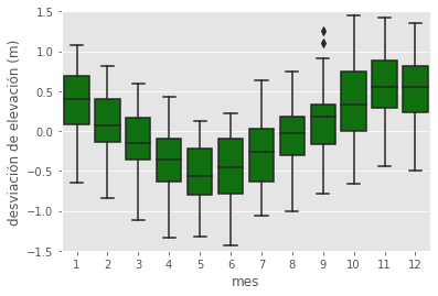
sns.boxplot(data=df, x='mes', y='nivel', color='g');
plt.ylim(-1.5, 1.5)
plt.xlabel('mes')
plt.ylabel('desviación de elevación (m)');
palette = sns.cubehelix_palette(light=.9, n_colors=len(df['año'].unique()))

sns.relplot(data=df, x="dda", y="nivel", hue="año", kind='line', palette=palette,
            height=5, aspect=1.5)
# Change x axis labelling to show months rather than just dda integers
# 0,365 for start of month; 15,380 for middle of month
plt.xticks(np.linspace(0,365,13)[:-1],
           ('Ene', 'Feb', 'Mar', 'Abr', 'May', 'Jun', 'Jul', 'Ago', 'Sep', 'Oct', 'Nov', 'Dic')
          );
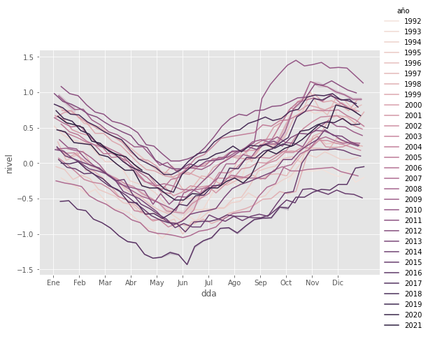
Nota: Para estas figuras, hay que eliminar los años incompletos – el primero y tipicamente el ultimo (a menos que la fecha mas reciente sea mediados de diciembre)
dfg = df.groupby('año')
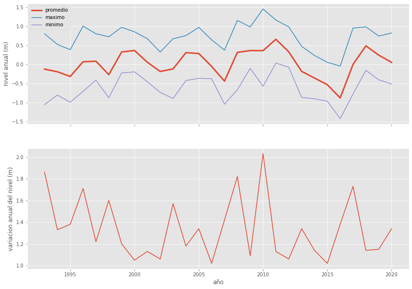
Una sola figura con el promedio, minimo y maximo anual
fig, ejes = plt.subplots(nrows=2, figsize=(14,10), sharex=True)

dfg.nivel.mean().iloc[1:-1].plot(ax=ejes[0], label='promedio', linewidth=3)
dfg.nivel.max().iloc[1:-1].plot(ax=ejes[0], label='maximo')
dfg.nivel.min().iloc[1:-1].plot(ax=ejes[0], label='minimo')
ejes[0].set_ylabel('nivel anual (m)')
ejes[0].legend()

dfheightrange = dfg.nivel.max().iloc[1:-1] - dfg.nivel.min().iloc[1:-1]
dfheightrange.plot(ax=ejes[1])
ejes[1].set_ylabel('variacion anual del nivel (m)');
Explorar lakepy
Incluyendo accesso a datos del Lago de Managua (Xolotlan)
import lakepy
Lago Nicaragua
lago_nica_lp = lakepy.search(name='%nicaragua%')
   id_No    source  lake_name
0    129  hydroweb  Nicaragua
1   1943    grealm  Nicaragua
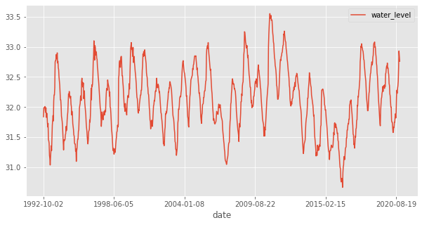
lago_nica_lp_grealm = lakepy.search(id_No=1943)
| id_No | lake_name | source | Type | Country | Continent | Resolution | grealm_database_ID | Satellite Observation Period | |
|---|---|---|---|---|---|---|---|---|---|
| 0 | 1943 | Nicaragua | grealm | open | Nicaragua | Central America | 10.0 | 351 | Sept 1992-present |
Reading lake level records from database...
La informacion que fue imprimida arriba es la misma que ahora esta disponible por medio de lago_nica_lp_grealm.metadata.
lago_nica_lp_grealm.data.tail()
| id_No | date | lake_name | water_level | |
|---|---|---|---|---|
| 1006 | 1943 | 2020-10-18 | Nicaragua | 32.43 |
| 1007 | 1943 | 2020-11-07 | Nicaragua | 32.64 |
| 1008 | 1943 | 2020-11-27 | Nicaragua | 32.93 |
| 1009 | 1943 | 2020-12-16 | Nicaragua | 32.85 |
| 1010 | 1943 | 2020-12-26 | Nicaragua | 32.76 |
lago_nica_lp_grealm.data.plot(x='date', y='water_level', figsize=(10,5));
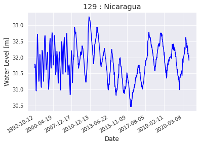
Comparar con los resultados de la fuente hydroweb
lago_nica_lp_hw = lakepy.search(id_No=129)
| id_No | lake_name | source | basin | status | country | end_date | latitude | longitude | identifier | start_date | |
|---|---|---|---|---|---|---|---|---|---|---|---|
| 0 | 129 | Nicaragua | hydroweb | San Juan | operational | Nicaragua | 2020-09-28 15:35 | 11.5 | -85.5 | L_nicaragua | 1992-10-12 11:31 |
Reading lake level records from database...
lago_nica_lp_hw.plot_timeseries(how='matplotlib')
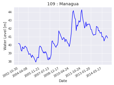
Lago Managua (Xolotlan)
lago_managua_lp = lakepy.search(name='%managua%')
| id_No | lake_name | source | basin | status | country | end_date | latitude | longitude | identifier | start_date | |
|---|---|---|---|---|---|---|---|---|---|---|---|
| 0 | 109 | Managua | hydroweb | San Juan | research | Nicaragua | 2015-01-26 20:12 | 12.35 | -86.35 | L_managua | 2002-10-30 22:47 |
Reading lake level records from database...
lago_managua_lp_hw = lakepy.search(id_No=109)
| id_No | lake_name | source | basin | status | country | end_date | latitude | longitude | identifier | start_date | |
|---|---|---|---|---|---|---|---|---|---|---|---|
| 0 | 109 | Managua | hydroweb | San Juan | research | Nicaragua | 2015-01-26 20:12 | 12.35 | -86.35 | L_managua | 2002-10-30 22:47 |
Reading lake level records from database...
lago_managua_lp_hw.plot_timeseries(how='matplotlib')